
More Information
Submitted: October 30, 2026 | Accepted: November 02, 2026 | Published: November 04, 2026
Citation: Iamrache L, Rekab K. Relative-distance Calibration for Spatial Relative-risk Forecasting: A Predictor–corrector Approach. J Community Med Health Solut. 2026; 7(2): 123-128. Available from:
https://dx.doi.org/10.29328/journal.jcmhs.1001087
DOI: 10.29328/journal.jcmhs.1001087
Copyright license: © 2026 Iamrache L, et al. This is an open access article distributed under the Creative Commons Attribution License, which permits unrestricted use, distribution, and reproduction in any medium, provided the original work is properly cited.
Keywords: Spatial relative risk; Relative absolute distance; Predictor–corrector; Expo-nential smoothing; Multiple linear regression; COVID-19 morbidity

Relative-distance Calibration for Spatial Relative-risk Forecasting: A Predictor–corrector Approach
Lyza Iamrache* and Kamel Rekab
Division of Computing, Analytics and Mathematics, School of Science and Engineering University of Missouri–Kansas City, Kansas City, Missouri, USA
*Corresponding author: Lyza Iamrache, Division of Computing, Analytics and Mathematics, School of Science and Engineering University of Missouri–Kansas City, Kansas City, Missouri, USA, Email: [email protected]
We investigate relative absolute distance as a calibration criterion for the spatial relative-risk predictor–corrector framework developed for COVID-19 morbidity data. The analysis retains seven observation intervals, the original regression and exponential-smoothing components, and the temporal training and forecast structure. Replacing cumulative squared-error loss with cumulative absolute relative distance changes the optimal smoothing weight from 0.38 to 0.35. The proposed method gives R2 = 0.955787, compared with R2 = 0.915 for the earlier method. This is an increase of 0.040787, or approximately 4.08 percentage points.
The relative-distance calibration achieved R2 = 0.955787, compared with R2 = 0.915 for the previously published squared-error calibration. Both methods were evaluated using the same observations and transformation. These findings suggest that the choice of calibration criterion influences predictive performance. The findings indicate that proportional-error calibration can alter the fitted predictor–corrector balance and improve agreement. Further validation on additional periods would strengthen the assessment of predictive performance.
Monitoring geographic variation in disease risk is central to public-health surveillance. Spatial scan statistics identify clusters with elevated or reduced relative risk [3], but the estimates obtained from cluster detection do not by themselves provide forecasts for future intervals. Iamrache, et al. [1] studied a predictor–corrector procedure combining an exponentially smoothed estimate with a regression-based correction to forecast spatial relative risks over successive intervals. Related predictor–corrector estimation of spatial-cluster relative risks was investigated by Bani-Yaghoub, et al. [2].
The choice of calibration loss influences which forecasts are preferred. Squared error emphasizes large absolute deviations, while a relative-error criterion measures the discrepancy as a proportion of the observed risk. When risks vary substantially across spatial units, these objectives need not select the same smoothing parameter or correction component.
This article evaluates a relative-distance calibration of the established predictor–corrector framework. The contribution is the loss function used for tuning and corrector selection; neither the underlying spatial scan procedure nor the Markov-chain formulation is redefined. We report the optimization results, interval-seven forecast errors, and a matched comparison with the published coefficient of determination. We investigate how replacing squared-error distance with absolute relative distance affects the smoothing parameter, correction-component selection, and seventh-interval forecasts. The underlying predictor–corrector framework, regression procedure, and exponential-smoothing recursion remain unchanged.
Study data
The source study examined U.S. COVID-19 morbidity over seven consecutive intervals between May 24, 2020, and March 12, 2023. Relative risks were obtained from spatial clusters identified by a Poisson spatial scan, with a maximum scanning window of 25% of the population at risk and significance assessed using 999 Monte Carlo replications. The present analysis uses the same interval-level relative-risk data and forecasting structure.
For componentwise calculations, entries must correspond to the same spatial units across intervals. Geographic alignment is necessary because pairing observations by vector position alone does not establish that they represent the same area. The relative-distance formula assumes positive observed risks. All observed relative-risk values used in the relative-distance calculations were examined and found to be strictly positive. Therefore, the proposed criterion is well-defined without adding a stabilizing constant to the denominator.
Predictor–corrector specification
Let Ti denote the vector of observed spatial relative risks at interval i. The predictor–corrector framework combines the most recent observation with a corrected estimate:
Let Ti denote the matrix of observed spatial relative risks at observation interval i, where i = I,…,7. The element Ti (m,n) represents the observed relative risk at spatial position (m,n). The same spatial arrangement is maintained across all observation intervals to ensure correspondence between observed and predicted values.
The predictor–corrector framework combines the most recent observation with a selected correction component:
(1)
The corrected estimate is chosen from a multiple-linear-regression estimate ( ) and an exponentially smoothed estimate ( ). The smoothing component draws on exponential-smoothing methods [4]. The smoothing recursion is
(2)
The recursion is initialized using , where comes from a linear regression of T2 on T1. For the sixth interval, the regression component fits T6 using T1 through T5. A shifted-predictor regression forecast provides a benchmark for interval seven. The smoothing recursion is initialized by setting , where is obtained from ordinary least-squares regression of T2 on T1. The fitted equation is
(3)
For the sixth interval, multiple linear regression estimates T6 from the five preceding relative-risk matrices. The fitted regression equation is
(4)
The regression coefficients are estimated using ordinary least squares by minimizing the sum of squared residuals across corresponding spatial observations. Both the regression and exponential-smoothing estimates provide candidate correction components, which are compared using the proposed relative-distance criterion. The regression fitting procedure remains unchanged from the original framework.
For each regression model, the coefficients are obtained by minimizing the sum of squared differences between the observed relative risks and their fitted values across corresponding spatial positions.
More generally, the use of alternative forecasting schemes as benchmarks is consistent with forecast-comparison research [5]. The forecasting procedure follows the predictor–corrector framework introduced by Iamrache et al. (2026). The observed relative-risk matrices are denoted by T1, T2,…T7 .
The regression estimate and the exponentially smoothed estimate are calculated using the same procedures as in the original study. The present analysis modifies only the distance criterion used to determine the optimal smoothing parameter and select the correction component.
Reference calibration
The original approach calibrates α by minimizing cumulative squared distance between smoothed estimates and observed relative risks over intervals three through six:
(5)
Using the relative-risk matrix notation, the reference squared-error distance is written as
(6)
(7)
The published analysis reported . The proposed calibration retains the same forecasting components and training intervals but changes the distance criterion.
Relative absolute distance
The present study introduces absolute relative distance as the calibration criterion for the predictor–corrector forecasting procedure.
In contrast to the squared-error criterion, which evaluates absolute prediction discrepancies on a squared scale, relative distance measures prediction discrepancies in proportion to the observed relative risks.
For the predicted relative-risk matrix and observed relative-risk matrix Ti, the distance is defined by
(8)
Here, represents the predicted relative risk at matrix position (m,n), and Ti (m,n) denotes the corresponding observed relative risk.
The proposed criterion aggregates componentwise absolute relative errors. Consequently, the total distance is not restricted to the interval [0,1] and may exceed one.
All observed relative-risk values used in the analysis were checked and found to be strictly positive. Therefore, the distance is well-defined without adding a constant to the denominator.
Unlike an average relative error, this criterion is the sum of the relative errors across all matrix entries. Consequently, the total relative distance is not restricted to the interval [0,1]and may exceed one.
All observed relative-risk values used in the present analysis were examined and found to be strictly positive. Therefore, the denominator is nonzero for every observation, and no adjustment to the denominator is required.
For paired forecast and observed vectors A and B, with Bj > 0, define the relative absolute distance as
(9)
Relative distance weights each absolute error by the magnitude of its observed risk. For example, a discrepancy of 0.5 corresponds to a 50% relative error when the observed risk is 1, but only 10% when it is 5.
All observed relative-risk values are strictly positive, so the relative-distance criterion is well-defined for the study data.
Calibration of the smoothing weight
The smoothing parameter is chosen by minimizing cumulative relative distance over the same four calibration intervals used by the reference approach:
(10)
The numerical implementation evaluates α on the grid 0.00,0.01,...,0.99. The smoothing parameter is calibrated over the closed interval [0,1]. The numerical search evaluates, α = 0.00,0.01,...,1.00, including both endpoints. Thus the reported optimum is a grid optimum rather than a claim of continuous global optimality. A finer search could assess the stability of the selected value.
Selection of the correction component
After estimating , compare the sixth-interval regression and smoothing candidates using the same relative-distance criterion. The regression candidate is selected when its distance is smaller; otherwise smoothing is selected:
(11)
The forecast for interval seven is then
(12)
The regression and exponential-smoothing candidates are compared using the observed relative-risk matrix from the sixth interval.
The candidate with the smaller absolute relative distance is selected as the correction component.
The seventh observation interval is excluded from both smoothing-parameter calibration and correction-component selection and is used only for forecast evaluation.
The sixth observation interval serves as the final calibration interval because it is the most recent observed interval available before forecasting interval seven. The regression and exponential-smoothing candidates are evaluated using the observed relative risks from interval six.
The seventh observation interval is reserved exclusively for forecast evaluation and does not influence parameter calibration or correction-component selection.
This modification affects calibration and corrector selection. The regression component itself remains an ordinary-least-squares model; it is not refitted using a relative-error regression objective.
Computational algorithm.
The complete forecasting procedure is summarized in the following steps.
1. Obtain the observed relative-risk matrices T1,...,T6.
2. Estimate using ordinary least-squares regression of T2 on T1.
3. For each candidate smoothing parameter α, initialize and recursively calculate for i = 3,...,6.
4. Calculate the cumulative relative-distance objective
5. Select the parameter α* minimizing D(α).
6. Estimate using multiple linear regression of T6 on T1,…,T5
7. Compare the regression and smoothing distances from T6. Select the candidate with the smaller distance as .
8. Compute the seventh-interval forecast:
9. Evaluate the forecast using the observed matrix T7, which was not used for calibration.
Forecast evaluation
The smoothing weight and correction component are selected using information through interval six. Interval seven is reserved for forecast evaluation. Forecast accuracy is summarized using total absolute relative distance and R2.
Let yj and denote the observed and predicted relative risks for matched spatial observation j, where J = 1,…,N. Forecast accuracy is assessed using the following error measures:
(13)
(14)
(15)
Here, N denotes the number of spatial observations used for forecast evaluation, yj denotes the observed relative risk, and denotes the corresponding predicted relative risk at spatial position j.
The MAE and RMSE are computed on the original relative-risk scale, whereas MARE measures the average absolute prediction error relative to the observed risk.
The coefficient of determination is computed across the spatial observations using
(16)
Where zj and represent the separately standardized logarithms of the observed and predicted relative risks, respectively, and denotes the mean of the standardized observed values.
The coefficient of determination is evaluated across corresponding spatial observations in the seventh interval.
The observed and predicted relative risks are logarithmically transformed and standardized separately before calculating R2.
The same transformation and evaluation procedure are applied to both calibration approaches to ensure comparability.
Optimization results
The initial regression of T2 on T1 gave an intercept of -0.141345 and slope of 0.918874. The cumulative relative-distance objective reached its grid minimum at α* = 0.35, with value 16.745848. The neighboring objective values were 16.747480 at α = 0.34 and 16.757976 at α = 0.36.
At α = 0.35; the interval-specific smoothing distances were 6.023482 for T3, 3.853101 for T4, 3.060555 for T5, and 3.808710 for T6. At interval six, the regression candidate achieved relative distance 3.512698, smaller than the smoothing distance of 3.808710. Accordingly, regression was selected as the correction component.
The fitted interval-six regression coefficients were - 6.173355 (intercept), - 0.299132 (T1), 5.566637 (T2), -0.224237 (T3), - 2.220742 (T4), and 3.353645 (T5). The resulting interval-seven forecast is
(17)
Interval-seven performance
For interval seven, the predictor–corrector forecast achieved a total absolute relative distance of 3.636899. Smoothing alone yielded 5.103426, and the shifted-regression benchmark yielded 48.822687. The proposed method achieved R2 = 0.955787.
The predictive performance of the proposed relative-distance calibration approach was evaluated using the seventh observation interval, which was reserved for forecast assessment.
The coefficient of determination, calculated using standardized logarithms of the observed and predicted relative risks, was R2 = 0.955787 (Figure 1).
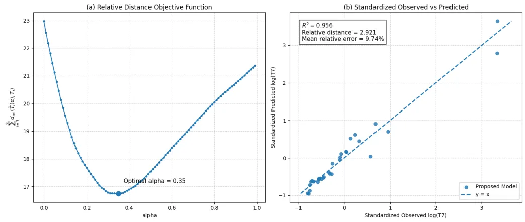
Figure 1: Relative-distance calibration and forecasting performance: (a) cumulative relative-distance objective with α* = 0.35; (b) observed versus predicted values with R2 = 0.955787.
On the original relative-risk scale, the mean absolute error was MAE = 0.491890, and the root mean squared error was RMSE = 1.573545.
The mean absolute relative error was MARE = 0.097350, corresponding to 9.7350%.
These results summarize the predictive accuracy of the proposed predictor–corrector approach for the seventh observation interval.
The observed and predicted relative-risk values for the seventh observation interval, together with the calibration objective values for all evaluated smoothing parameters, are provided in the Supplementary Material to facilitate independent verification and reproducibility.
Numerical comparison (Table 1)
| Table 1: Comparison of reported calibration and evaluation results. | ||
| Measure | Published calibration | Relative-distance calibration |
| Calibration loss | Squared error | Absolute relative distance |
| Optimal a | 0.38 | 0.35 |
| Reported | 0.915 | 0.955787 |
| R2 difference | — | +0.04787 |
Both calibration approaches were implemented using the same dataset, spatial units, regression and exponential-smoothing procedures, and forecasting framework.
The only modification was the distance criterion used for parameter calibration and correction-component selection.
Both approaches were evaluated using the same seventh-interval observations and the same definition of R2, calculated from separately standardized logarithmic relative risks.
The squared-error calibration yielded R2 = 0.915, whereas the proposed relative-distance calibration achieved R2 = 0.955787.
This corresponds to an increase of approximately 4.08 percentage points in the coefficient of determination.
Sensitivity analysis
The sensitivity of the proposed relative-distance calibration was examined by varying the resolution of the smoothing-parameter search grid.
The original grid with increments of 0.01 yielded an optimal smoothing parameter of α* = 0.35. Refining the grid to increments of 0.001 produced α* = 0.351, while a finer increment of 0.0001 yielded α* = 0.3518 (Table 2).
| Table 2: Sensitivity of the optimal smoothing parameter to grid resolution. | ||
| Grid step | Optimal α | Minimum objective |
| 0.01 | 0.3500 | 16.745848 |
| 0.001 | 0.3510 | 16.745710 |
| 0.0001 | 0.3518 | 16.745603 |
These results indicate that the selected smoothing parameter is relatively stable with respect to grid resolution. The search included both endpoints, α = 0 and α = 1 , and neither endpoint minimized the calibration objective.
All observed relative-risk values in the present study were strictly positive, ensuring that the proposed relative-distance criterion was well-defined without requiring any adjustment to the denominator. Although no zero denominators occurred in this application, the influence of very small positive relative-risk values may be investigated in future studies.
The analysis demonstrates that the loss function is a substantive modeling choice in spatial relative-risk forecasting. Squared error assigns increasing weight to large absolute deviations, whereas absolute relative distance measures proportional discrepancies. These criteria may lead to different parameter values even when the regression and smoothing structures and input observations are unchanged.
For the present data, relative-distance calibration selected instead of the previously reported squared-error weight of 0.38. The regression component was preferred to exponential smoothing at interval six. The resulting predictor–corrector forecast had a lower total relative distance on interval seven than either of the two reported individual benchmark forecasts.
The proposed method achieved R2 = 0.955787, compared with R2 = 0.915 for the earlier method, an increase of 0.040787 (4.08 percentage points).
The relative-distance calibration yielded a reported coefficient of determination of R2 = 0.955787. A direct comparison with the previously published coefficient of determination requires the same spatial observations, evaluation transformations, and definition of R2. The difference supports improved agreement for the reported evaluation, although additional test periods and error measures would strengthen the comparison.
Relative-error objectives also deserve care when observed values are very small, because their contributions may become disproportionately large. Moreover, the correction component is selected using its sixth-interval fit, and the empirical forecast assessment centers on a single held-out interval. Evaluations across additional temporal splits and explicit paired comparisons under several losses would provide stronger evidence of predictive robustness.
We presented a relative-distance calibration of an established spatial relative-risk predictor–corrector forecasting procedure. The modification preserves the regression and exponential-smoothing components while selecting the smoothing weight and correction component by absolute relative distance. The estimated smoothing weight was 0.35, and regression was selected as the sixth-interval correction component.
The proposed method achieved R2 = 0.955787, compared with R2 = 0.915 for the earlier squared-error calibration.
The seventh-interval forecast also yielded MAE = 0.491890, RMSE = 1.573545, and MARE = 9.7350%.
These findings suggest that the choice of calibration criterion can influence forecasting accuracy within the predictor–corrector framework.
The interval-seven forecast attained total relative distance 3.636899. The proposed method achieved R2 = 0.955787, compared with 0.915 for the earlier squared-error calibration. These findings support further study of proportional-error objectives for spatial risk prediction.
- Iamrache L, Rekab K, Bani-Yaghoub M, Pluta J, Mehailia A. A Markov chain modeling approach for predicting relative risks of spatial clusters in public health. Discover Public Health. 2026;23:748. Available from: https://doi.org/10.1186/s12982-026-02009-7.
- Bani-Yaghoub M, Rekab K, Pluta J, Tabharit S. Estimating the relative risks of spatial clusters using a predictor-corrector method. Mathematics. 2025;13(2):180.
- Kulldorff M. A spatial scan statistic. Communications in Statistics–Theory and Methods. 1997;26(6):1481–1496.
- Brown RG. Exponential Smoothing for Predicting Demand. Arthur D. Little; 1956.
- Clark TE, McCracken MW. Improving forecast accuracy by combining recursive and rolling forecasts. International Economic Review. 2009;50(2):363–395.